38) Stiff Equations

Last time

• Ordinary differential equations (ODE)

• Stability of ODEs

• Explicit methods for solving ODE

• Linear Stability Analysis

• Numerical stability of ODEs

Today

1. The \(\theta\) methods

2. \(A\)-stability

3. \(L\)-stability

4. Examples of PDEs

5. Stiff equations

6. Adaptive time integrators (or time stepping schemes)

using LinearAlgebra
using Plots
default(linewidth=4, legendfontsize=12)
using LaTeXStrings

struct RKTable
    A::Matrix
    b::Vector
    c::Vector
    function RKTable(A, b)
        s = length(b)
        A = reshape(A, s, s)
        c = vec(sum(A, dims=2))
        new(A, b, c)
    end
end

function rk_stability(z, rk)
    s = length(rk.b)
    1 + z * rk.b' * ((I - z*rk.A) \ ones(s))
end

rk4 = RKTable([0 0 0 0; .5 0 0 0; 0 .5 0 0; 0 0 1 0], [1, 2, 2, 1] / 6)
heun = RKTable([0 0; 1 0], [.5, .5])
Rz_theta(z, theta) = (1 + (1 - theta)*z) / (1 - theta*z)

function ode_rk_explicit(f, u0; tfinal=1, h=0.1, table=rk4)
    u = copy(u0)
    t = 0.
    n, s = length(u), length(table.c)
    fY = zeros(n, s)
    thist = [t]
    uhist = [u0]
    while t < tfinal
        tnext = min(t+h, tfinal)
        h = tnext - t
        for i in 1:s
            ti = t + h * table.c[i]
            Yi = u + h * sum(fY[:,1:i-1] * table.A[i,1:i-1], dims=2)
            fY[:,i] = f(ti, Yi)
        end
        u += h * fY * table.b
        t = tnext
        push!(thist, t)
        push!(uhist, u)
    end
    thist, hcat(uhist...)
end

ode_rk_explicit (generic function with 1 method)

Ordinary Differential Equations

Given initial condition \(y_0 = y(t=0)\), find \(y(t)\) for \(t > 0\) that satisfies

\[ y' \equiv \dot y \equiv \frac{\partial y}{\partial t} = f(t, y) \]

Application	\(y\)	\(f\)
Orbital dynamics	position, momentum	conservation of momentum
Chemical reactions	concentration	conservation of atoms
Epidemiology	infected/recovered population	transmission and recovery

• \(y\) can be a scalar or a vector

Recap on solving differential equations

Recap on linear equations

\[ y' = A(t) y + \text{sink}(t)/\text{source}(t)\]

• Autonomous if \(A(t) \equiv A\) and source independent of \(t\): \( y' = A y + \text{sink}/\text{source}\)

• Non-autonomous otherwise

• Suppose \(y\) and \(a = A\) are scalars:

\[ y' = a y\]

then there is an an analytic solution:

\[y(t) = e^{at} y_0\]

• We can do the same for systems

\[ y(t) = e^{A t} y_0 \]

But what does it mean to exponentiate a matrix?

Taylor series again!

\[ e^A = 1 + A + \frac{A^2}{2} + \frac{A^3}{3!} + \dotsb \]

where here \(1\) means the identity matrix \(I\), and there are many practical ways to compute it (a paper co-authored by the founder of MATLAB).

Exponentiate a diagonalizable matrix

Suppose that the diagonalization \(A = X \Lambda X^{-1}\) exists, how do we derive a finite expression for the matrix exponential of \(A\), i.e., \(e^A\), using the scalar exp function?

Solution:

We have:

\[ e^A = 1 + A + \frac{A^2}{2} + \frac{A^3}{3!} + \dotsb \]

\[A^n = (X \Lambda X^{-1})^n = X \Lambda X^{-1} \cdot X \Lambda X^{-1} \cdot X \Lambda X^{-1} \cdot \ldots \cdot X \Lambda X^{-1} = X \Lambda^n X^{-1}\]

Thus,

\[ e^A = X X^{-1} + X \Lambda X^{-1} + X \Lambda^2 X^{-1}/2 + \dots \]

Factoring out the \(X\) and \(X^{-1}\) on the left and right gives:

\[e^A = X (I + \Lambda + \Lambda^2/2 + \dots) X^{-1} = X e^{\Lambda}X^{-1}.\]

Stability of ODEs

A solution of the ODE

\[ y' = f(t, y) \]

is stable if for every \(\varepsilon > 0\) there is a \(\delta > 0\) s. t. if \(\hat y(t)\) satisfies the ODE and \( \hat y(t_0) − y(t_0) \leq \delta\) then \(|| \hat y(t) - y(t)|| \leq \varepsilon\) for all \(t \geq t_0\),

that is, it rules out exponential divergence if initial value is perturbed.

There are different scenarios:

• Asymptotically stable solution: \(|| \hat y(t) - y(t)|| \rightarrow 0 \) as \(t \rightarrow \infty\)

• Stable solution, but not asymptotically so:

• Unstable solution:

Determining stability

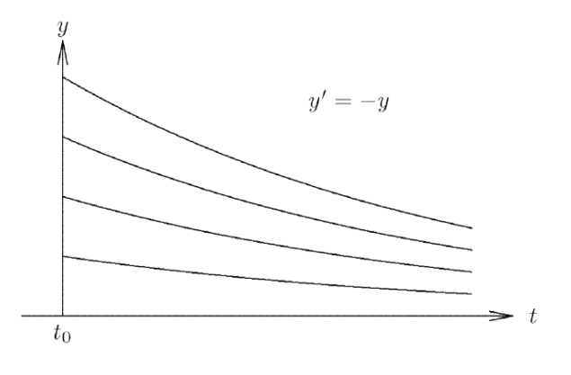
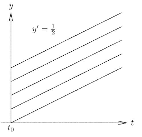
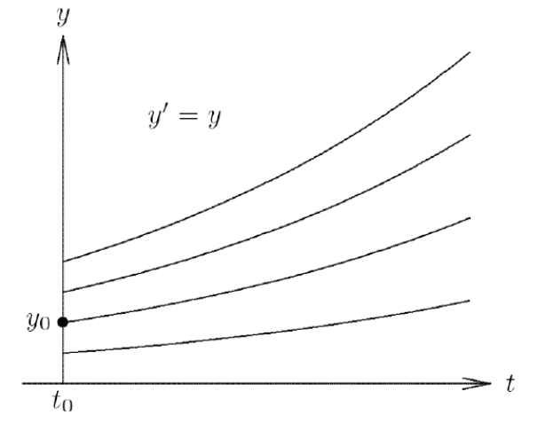
To determine stability of an ODE, we think of the simpler case of a linear, homogenous system \( y' = A y \), or even simpler, where we have only a constant \(\lambda\) multiplied by \(y\). This is called a “test” equation:

\[ y' = \lambda y . \]

We know this has an analytic solution \(y(t) = y_0 e^{\lambda t}\), for an initial condition \(y(0)=y_0\).

• If \(\lambda > 0\), exponential divergence: every solution is unstable.

• \(\lambda < 0\), asymptotical stability: every solution is stable as \(t \rightarrow \infty\).

• If \(\lambda \) is complex:

  • \(e^{\lambda t} = e^{a t} (\cos(b t ) + i \sin( b t))\)

  • \(Re(\lambda) = a\). This is the oscillating component multiplied by a real amplification factor

    • \(Re(\lambda) > 0\): unstable (solution grows)

    • \(Re(\lambda) < 0\): stable (solution decays)

    • \(Re(\lambda) = 0\): oscillating (solution oscillates)

Recap on explicit methods for solving ODEs: Forward Euler method

The simplest method for solving

\[y'(t) = f(t,y)\]

is to use numerical differentiation to approximate the derivative.

Recall: We know the definition of the difference quotient from Calculus:

\[y' = \lim_{h\to 0} \frac{y(t+h) - y(t)}{h}\]

Hence, we can use a forward difference formula:

\[ \frac{\partial {y^n}^F}{\partial t} \approx \frac{ y^{n+1} - y^{n}}{h} + O(h) \equiv \frac{ y^{n+1} - y^{n}}{\Delta t} + O(\Delta t) \]

this is a first-order approximation, where \(h \equiv \Delta t\) is the step size, and we have approximated the time domain (temporal axis) with uniform grid spacing \(\Delta t\), so that \(y^n = n \Delta t\), for \(n = 0, \ldots, N\).

When \(n=0\) we use the initial condition given: \(y(t=0)=y(0)=y_0\)

\[ y' \approx \frac{y(h) - y(0)}{h} \]

which yields

\[ y' \approx \frac{y(h) - y(0)}{h} = f(0, y(0)) \]

Hence, we have the solution estimate

\[ \tilde y(h) = y(0) + h f(0, y(0)) \]

Let’s now use again the simplest linear ODE there exists, the “test” equation:

\[ y' = \lambda y . \]

For \(n=0\) we obtain the solution at new time step (\(n=1\)) knowing all information that is given by the initial condition:

\[ y^{1} = y^0 + h \lambda y^0 , \]

For multiple steps, \((n \geq 1))\), we obtain the recurrence relation:

\[ y^{n+1} = y^n + h \lambda y^n , \]

\[ y^{n+1} = \left(1 + h \lambda \right) y^n . \]

If we apply this repeatedly, we obtain the relation:

\[ y^{n+1} = \left(1 + h \lambda \right)^{n+1} y^0 . \]

Example:

Let’s try this on a scalar problem

\[ y' = -k (y - \cos t) \]

where \(k\) is a parameter controlling the rate at which the solution \(y(t)\) is pulled toward the curve \(\cos t\).

# Forward Euler ODE time-stepper
function ode_euler(f, y0; tfinal=10., h=0.1)
    y = copy(y0)
    t = 0.
    thist = [t]
    yhist = [y0]
    while t < tfinal
        tnext = min(t+h, tfinal)
        h = tnext - t
        y += h * f(t, y) # explicit step
        t = tnext
        push!(thist, t)
        push!(yhist, y)
    end
    thist, hcat(yhist...)
end

ode_euler (generic function with 1 method)

f1(t, y; k=10) = -k * (y .- cos(t))

thist, yhist = ode_euler(f1, [1.], tfinal=20, h=.2)
plot(thist, yhist[1,:], marker=:circle, label = "Forward Euler")
plot!(cos, label = L"\cos(x)")

Forward Euler on a linear system

If we have a system of ODEs:

\[ \dot{\mathbf{y}} = A \mathbf{y} \]

For example, a system of two first-order linear ODEs:

(21)\[\begin{align} y_1' &= y_2\\ y_2' &= - y_1\\ \end{align}\]

In matrix form:

\[\begin{split} \begin{bmatrix} y_1 \\ y_2 \end{bmatrix}' = \begin{bmatrix} 0 & 1 \\ -1 & 0 \end{bmatrix} \begin{bmatrix} y_1 \\ y_2 \end{bmatrix}\end{split}\]

f2(t, y) = [0 1; -1 0] * y

thist, yhist = ode_euler(f2, [0., 1], h=.1, tfinal=80)
scatter(thist, yhist', label = [L"y_1" L"y_2"])
plot!([cos, sin], label = [L"\cos(x)" L"\sin(x)"])

eigvals([0 1; -1 0])

2-element Vector{ComplexF64}:
 0.0 - 1.0im
 0.0 + 1.0im

Recap on Runge-Kutta 4

thist, yhist = ode_rk_explicit(f2, [0., 1], h=0.5, tfinal=50)
scatter(thist, yhist', label = [L"y_1" L"y_2"])
plot!([cos, sin], label = [L"\cos(x)" L"\sin(x)"])

• Apparently it is possible to integrate this system using large time steps.

• This method evaluates \(f(t)\) four times per step, so the cost is about equal when the step size \(h\) is 4x larger than forward Euler.

But let’s run it again with a larger step size

thist, yhist = ode_rk_explicit(f2, [0., 1], h=2.9, tfinal=50)
scatter(thist, yhist', label = [L"y_1" L"y_2"])
plot!([cos, sin], size=(800, 500), label = [L"\cos(x)" L"\sin(x)"])

Recap on stability

To analyze stability, we use the Linear Stability Analysis (LSA).

Linear Stability Analysis

Why did Euler diverge (even if slowly) while RK4 solved this problem accurately?

And why do both methods diverge if the step size is too large?

We can understand the convergence of methods by analyzing the test problem

\[ y' = \lambda y \]

for different values of \(\lambda\) in the complex plane.

One step of the Euler method with step size \(h\) maps

\[ y \to y + h \lambda y = \underbrace{(1 + h \lambda)}_{R(h \lambda)} y .\]

For many (\(n \geq 1 \)) steps, we have:

\[ y^{n+1} = y^n + h \lambda y^n . \]

Hence, we obtain the recurrence relation:

\[ y^{n+1} = \underbrace{(1 + h \lambda)}_{R(h \lambda)} y^n, \]

where \(R(h \lambda)\) is called the recurrence relation or growth/amplification factor.

Our solution will stay bounded, that means the numerical scheme is stable if and only if

\[|R(h \lambda)| \leq 1 . \]

Let’s look at examples when this map causes solutions to “blow up” or to be stable.

function plot_stability(Rz, method; xlim=(-3, 2), ylim=(-1.5, 1.5))
    x = xlim[1]:.02:xlim[2]
    y = ylim[1]:.02:ylim[2]
    plot(title="Stability region: $method", aspect_ratio=:equal, xlim=xlim, ylim=ylim)
    heatmap!(x, y, (x, y) -> abs(Rz(x + 1im*y)), c=:bwr, clims=(0, 2))
    contour!(x, y, (x, y) -> abs(Rz(x + 1im*y)), color=:black, linewidth=2, levels=[1.])
    plot!(x->0, color=:black, linewidth=1, label=:none)
    plot!([0, 0], [ylim...], color=:black, linewidth=1, label=:none)
end

plot_stability (generic function with 1 method)

plot_stability(z -> 1 + z, "Forward Euler")

This is a complex \(z = \lambda h \) (or \( z =\lambda \Delta t\))-plane.

Stability for RK4

plot_stability(z -> rk_stability(4z, rk4), "RK4")

Stability for Heun’s method

plot_stability(z -> rk_stability(2z, heun), "Heun's method")

Recap on implicit methods: Backward Euler

Recall that one forward Euler step is

\[ \tilde y(h) = y(0) + h f(0, y(0)) . \]

This can be evaluated explicitly; all the terms on the right hand side are known so the approximation \(\tilde y(h)\) is computed merely by evaluating the right hand side.

Let’s consider an alternative, backward Euler (or “implicit Euler”).

Recall the forward difference formula:

\[ \frac{\partial {y^n}^F}{\partial t} \approx \frac{ y^{n+1} - y^{n}}{h} + O(h) \equiv \frac{ y^{n+1} - y^{n}}{\Delta t} + O(\Delta t) \]

If instead we use the backward difference formula:

\[ \frac{\partial {y^{n}}^B}{\partial t} \approx \frac{ y^{n} - y^{n-1}}{h} + O(h) \equiv \frac{ y^{n} - y^{n-1}}{\Delta t} + O(\Delta t) \]

When \(n=1\) we use the initial condition given: \(y(t=t_0=0)=y(0)=y_0\)

\[ y'(t=t_1) \approx \frac{y(h) - y(0)}{h} \]

which yields

\[ y'(t=t_1) \approx \frac{y(h) - y(0)}{h} = f(t=t_1, y(t=t_1)) \]

which yields to the solution estimate

\[ \tilde y(h) = y(0) + h f(h, \tilde y(h)) . \]

This is a (generally) nonlinear equation for \(\tilde y(h)\).

Stability of backward Euler

For the test equation

\[ y' = \lambda y, \]

at the first time step, the backward Euler method is

\[ \tilde y(h) = y(0) + h \lambda \tilde y(h), \]

or

\[ \left(1 - h \lambda\right) \tilde y(h) = y(0) , \]

hence

\[ \tilde y(h) = \underbrace{\left( \frac{1}{1 - h \lambda}\right)}_{R(h\lambda)} y(0) . \]

For many steps, \((n \geq 1)\), we obtain:

\[ y^{n+1} = y^n + h \lambda y^{n+1} . \]

Hence, we obtain the recurrence relation:

\[ \left( 1 - h \lambda \right) y^{n+1} = y^n, \]

\[ y^{n+1} = \underbrace{\left( \frac{1}{1 - h \lambda}\right)}_{R(h\lambda)} y^n. \]

If we apply this repeatedly, we obtain:

\[ y^{n+1} = \left( \frac{1}{1 - h \lambda } \right)^{n+1} y^0. \]

We see that to have stability for the Backward Euler scheme we need:

\[ \left| \frac{1}{1 - h \lambda } \right| \leq 1 . \]

plot_stability(z -> 1/(1-z), "Backward Euler")

We can see that the stability region is for \(h \lambda\) anywhere in the left half complex plane, i.e., for any \(h>0\) when \(Re(\lambda)<0\).

• This means that if the problem of interest is stable \(\Rightarrow\) Backward Euler is unconditionally stable, i.e., stable for any positive step size \(h\).

Computing with implicit methods

\[ \tilde y(h) = y(0) + h f\big(\tilde y(h) \big) \]

• Linear solve for linear problem

• Nonlinear (often Newton) solve for nonlinear problem

• Need Jacobian or finite differencing

Recap on stability of midpoint (Crank-Nicolson) scheme

For the test equation

\[y' = \lambda y, \]

one step of the Crank-Nicolson scheme is

\[ \frac{y(h) - y(0)}{h} = \frac{1}{2} \left( f( y(0)) + f(y(h)) \right), \]

which leads to the solution estimate

\[ \tilde y(h) = y(0) + h \frac{1}{2} \left( f( y(0)) + f(\tilde y(h)) \right) . \]

We use the test problem:

\[ y' = \lambda y , \]

and we obtain:

\[ \tilde y(h) = y(0) + \frac{h \lambda}{2} y(0) + \frac{h \lambda}{2} \tilde y(h) , \]

which we can rearrange:

\[ \left(1 - \frac{h \lambda}{2} \right) \tilde y(h) = \left(1 + \frac{h \lambda}{2} \right) y(0) , \]

\[ \tilde y(h) = \left(\frac{ 1 + \frac{h \lambda}{2} }{1 - \frac{h \lambda}{2}} \right) y(0) . \]

For many steps, \((n \geq 1)\), we obtain:

\[ y^{n+1} = \left(\frac{ 1 + \frac{h \lambda}{2} }{1 - \frac{h \lambda}{2}} \right) y^n . \]

If we apply this repeatedly, we obtain:

\[ y^{n+1} = {\underbrace{\left(\frac{ 1 + \frac{h \lambda}{2} }{1 - \frac{h \lambda}{2}} \right)}_{R(h\lambda)}}^{n+1} y^0. \]

We see that to have stability for the Crank-Nicolson scheme we need:

\[ \left| \frac{ 1 + \frac{h \lambda}{2} }{1 - \frac{h \lambda}{2}} \right| \leq 1 . \]

plot_stability(z -> Rz_theta(z, .5), "Midpoint method")

Again, similarly to the case for Backward Euler, we can see here that the stability region is for \(h \lambda\) anywhere in the left half complex plane, i.e., for any \(h>0\) when \(Re(\lambda)<0\).

• This means that if the problem of interest is stable \(\Rightarrow\) Crank-Nicolson is unconditionally stable, i.e., stable for any positive step size \(h\).

1. The \(\theta\) methods

Forward and backward Euler are bookends of the family known as \(\theta\) methods, with Crank-Nicolson (or midpoint) exactly in the middle.

We can express a family of methods with the parameter \(\theta\). One step of the \(\theta\)-method looks like this:

\[ \tilde u(h) = u(0) + h f\Big(\theta h, \theta\tilde u(h) + (1-\theta)u(0) \Big) \]

which, for linear problems, is solved as

\[ (I - h \theta A) u(h) = \Big(I + h (1-\theta) A \Big) u(0) . \]

\(\theta=0\) is explicit Euler, \(\theta=1\) is implicit Euler, and \(\theta=1/2\) is the midpoint/trapezoid or Crank-Nicolson method (equivalent for linear problems).

The stability function (or growth/amplification factor) in this case is:

\[ R(z) = \frac{1 + (1-\theta)z}{1 - \theta z}, \]

where we have defined \(z= h \lambda\).

Rz_theta(z, theta) = (1 + (1-theta)*z) / (1 - theta*z)
theta = .5
plot_stability(z -> Rz_theta(z, theta), "\$\\theta=$theta\$",
    xlim=(-20, 1))

\(\theta\) method for the oscillator

# θ scheme: θ=0 is explicit (forward) Euler, θ=1 is implicit (backward) Euler, θ=0.5 is Crank-Nicolson
function ode_theta_linear(A, u0; forcing=zero, tfinal=1, h=0.1, theta=.5)
    u = copy(u0)
    t = 0.
    thist = [t]
    uhist = [u0]
    while t < tfinal
        tnext = min(t+h, tfinal)
        h = tnext - t
        rhs = (I + h*(1-theta)*A) * u .+ h*forcing(t+h*theta)
        u = (I - h*theta*A) \ rhs
        t = tnext
        push!(thist, t)
        push!(uhist, u)
    end
    thist, hcat(uhist...)
end

ode_theta_linear (generic function with 1 method)

# Test on oscillator
A = [0 1; -1 0]
theta = .5
thist, uhist = ode_theta_linear(A, [0., 1], h=.6, theta=theta, tfinal=20)
scatter(thist, uhist', label = [L"y_1" L"y_2"], title = L"\theta = 0.5")
plot!([cos, sin], label = [L"\cos(x)" L"\sin(x)"])

• This is called dispersion: the approximated wave is shifted laterally relative to the actual solution, but its height is not damped.

• Instead, numerical dissipation is when there is amplitude damping of the numerical solution as compared to the exact solution.

\(\theta\) method for the cosine decay

k = 500000
theta = .7
thist, uhist = ode_theta_linear(-k, [.2], forcing=t -> k*cos(t), tfinal=5, h=.1, theta=theta)
scatter(thist, uhist[1,:], title="\$\\theta = $theta\$", label = L"\theta = 0.7 \textrm{ scheme}")
plot!(cos, size=(800, 500))

• It starts rough but then it approximates the exact solution very closely, with no dispersion or dissipation.

• Next we are going to talk about different stability classes and the \(\theta\) method

2. \(A\)-stability

A method is \(A\)-stable if the stability region

\[ \{ z : |R(z)| \le 1 \} \]

contains the entire left half plane

\[ \Re[z] \le 0 .\]

This means that the method can take arbitrarily large time steps without becoming unstable (diverging) for any problem that is indeed physically stable.

3. \(L\)-stability

A time integrator with stability function \(R(z)\) is \(L\)-stable if

\[ \lim_{z\to\infty} R(z) = 0 .\]

That is, \(L\)-stability is a stronger property, for which the solution approaches zero in a single step as the step size goes to infinity.

For the \(\theta\) method, we have

\[ \lim_{z\to \infty} \frac{1 + (1-\theta)z}{1 - \theta z} = \frac{1-\theta}{\theta} . \]

Evidently only \(\theta=1\) is \(L\)-stable.

4. Examples of PDEs

Heat equation as linear ODE

\[ \frac{\partial u}{\partial t} = \frac{\partial^2 u}{\partial x^2} \]

on \([-1,1]\), with an initial condition \(u(x,t=0) = u_0 = e^{-200x^2}\), and periodic boundary conditions: \(u(-1)=u(1)\).

Although this is an example of an Initial Boundary Value Problem, as this is a Partial Differential Equation (PDE), as it has partial derivatives in both time \(t\) and space \(x\), we are going to analyze it here as a linear ODE, in the sense that it is linear in \(u\). In fact, the dependent variable \(u\) and its derivatives only appear to the first power, meaning there are no squared terms or nonlinear functions of the derivative of \(u\).

• How do different \(\theta \in [0, 1]\) compare in terms of stability?

• Are there artifacts even when the solution is stable?

using Pkg
Pkg.add("SparseArrays")
using SparseArrays

function heat_matrix(n)
    dx = 2 / n
    rows = [1]
    cols = [1]
    vals = [0.]
    wrap(j) = (j + n - 1) % n + 1
    for i in 1:n
        append!(rows, [i, i, i])
        append!(cols, wrap.([i-1, i, i+1]))
        append!(vals, [1, -2, 1] ./ dx^2)
    end
    sparse(rows, cols, vals)
end
heat_matrix(5)

   Resolving package versions...

  No Changes to `~/.julia/environments/v1.10/Project.toml`
  No Changes to `~/.julia/environments/v1.10/Manifest.toml`

┌ Warning: Circular dependency detected.
│ Precompilation will be skipped for dependencies in this cycle:
│  ┌ Symbolics → SymbolicsForwardDiffExt
│  └─ Symbolics → SymbolicsPreallocationToolsExt
└ @ Pkg.API.Precompilation ~/julia-1.10.10/share/julia/stdlib/v1.10/Pkg/src/precompilation.jl:583

5×5 SparseMatrixCSC{Float64, Int64} with 15 stored entries:
 -12.5     6.25     ⋅       ⋅      6.25
   6.25  -12.5     6.25     ⋅       ⋅ 
    ⋅      6.25  -12.5     6.25     ⋅ 
    ⋅       ⋅      6.25  -12.5     6.25
   6.25     ⋅       ⋅      6.25  -12.5

n = 200
A = heat_matrix(n)
x = LinRange(-1, 1, n+1)[1:end-1]
u0 = exp.(-200 * x .^ 2)
@time thist, uhist = ode_theta_linear(A, u0, h=.1, theta=0.5, tfinal=1); # try to change theta
nsteps = size(uhist, 2)
plot(x, uhist[:, 1:5], title = L"\theta = 0.5", xlabel = "x", ylabel = "u(x,t)") # plot only the first 5 time-steps

  1.532751 seconds (3.60 M allocations: 247.916 MiB, 4.76% gc time, 99.93% compilation time)

Example: Advection as a linear ODE

\[ \frac{\partial u}{\partial t} = - c \frac{\partial u}{\partial x} \]

on \([-1,1]\), with an initial condition \(u(x,t=0) = u_0 = e^{-9x^2}\), and periodic boundary conditions: \(u(-1)=u(1)\).

Here \(u(x,t)\), \(x \in \mathbb{R}\) is a scalar (wave), advected by a nonezero constant \(c\) during time \(t\). The sign of \(c\) characterise the direction of wave propagation. If \(c>0\), the wave propagates in the positive direction of \(x\)-axis. On the other hand, if \(c<0\) then the wave propagates to the negative direction of \(x\)-axis. The mangitude of \(c\) tells us how fast the wave propagates. The exact solution of this equation is given by its initial value. Assuming that the initial condition is given as \(u_0(x,t)= u(x,0)\), then the exact solution of equation is \(u(x,t) = u_0 (x-ct)\).

function advect_matrix(n; upwind=false)
    dx = 2 / n
    rows = [1]
    cols = [1]
    vals = [0.]
    wrap(j) = (j + n - 1) % n + 1
    for i in 1:n
        append!(rows, [i, i])
        if upwind # in this case, use upwind for the spatial derivative
            append!(cols, wrap.([i-1, i]))
            append!(vals, [1., -1] ./ dx)
        else # in this case, use a centered difference for the spatial derivative
            append!(cols, wrap.([i-1, i+1]))
            append!(vals, [1., -1] ./ 2dx)
        end
    end
    sparse(rows, cols, vals)
end
advect_matrix(5)

5×5 SparseMatrixCSC{Float64, Int64} with 11 stored entries:
  0.0   -1.25    ⋅      ⋅     1.25
  1.25    ⋅    -1.25    ⋅      ⋅ 
   ⋅     1.25    ⋅    -1.25    ⋅ 
   ⋅      ⋅     1.25    ⋅    -1.25
 -1.25    ⋅      ⋅     1.25    ⋅ 

• Question: What do you expect to happen to the shape of the blob with time?

• Answer: It should be preserved, since there is only advection (transport along a flow), and no diffusion (spread).

n = 50
A = advect_matrix(n, upwind=false) # uses a centered scheme
x = LinRange(-1, 1, n+1)[1:end-1]
u0 = exp.(-9 * x .^ 2)
@time thist, uhist = ode_theta_linear(A, u0, h=.04, theta=1, tfinal=1.); # run for 25 time steps in total
nsteps = size(uhist, 2)
plot(x, uhist[:, 1:(nsteps÷8):end], title = L"\theta = 1", xlabel = "x", ylabel = "u(x,t)") # plot solution at every 3 time steps

  0.087930 seconds (54.95 k allocations: 5.674 MiB, 98.13% compilation time)

• A lot of numerical dissipation!

• That is clearly not what happens, and changing theta doesn’t improve the situation.

• It looks like our discretization method somehow introduced an artifact, dissipation, independently of the method we use for the temporal evoluation of the solution.

• However, there is no catastrophic growth of the solution if you set tfinal to some large value (try it!), even if theta is set to less than \(0.5\).

• To demonstrate, below I plot the spectrum of the \(A\)-matrix produced by the upwind discretization.

Spectrum of operators

theta=.5  # Change this if you like
h = .1 # Change this if you like
plot_stability(z -> Rz_theta(z, theta), "\$\\theta=$theta, h=$h\$, advection equation")
ev = eigvals(Matrix(h*advect_matrix(20, upwind=true)))
scatter!(real(ev), imag(ev), label = "eigenvalues")

n = 50
A = advect_matrix(n, upwind=false)
x = LinRange(-1, 1, n+1)[1:end-1]
u0 = exp.(-9 * x .^ 2)
@time thist, uhist = ode_theta_linear(A, u0, h=.1, theta=0.5, tfinal=1.); # run for 25 time steps in total
nsteps = size(uhist, 2)
plot(x, uhist[:, 1:(nsteps÷8):end], title = L"\theta = 0.5") # plot solution at every 3 time steps

  0.029570 seconds (18.16 k allocations: 1.958 MiB, 98.42% compilation time)

• The \(\lambda\) values are clearly distributed differently, and in a way that restricts our choices for theta. Now we have to pick \(\theta \geq 0.5\) for temporal stability. See the spectrum below.

• Question: Why would a choice of theta restricted to larger values be undesirable?

theta=0. # Change this if you like
h = .01 # Change this if you like
plot_stability(z -> Rz_theta(z, theta), "\$\\theta=$theta, h=$h\$, advection equation")
ev = eigvals(Matrix(h*advect_matrix(50, upwind=false)))
scatter!(real(ev), imag(ev), label = "eigenvalues")

• The bottom line is that both of these spatial (and temporal) discretizations are bad, but for different reasons.

• The dissipation issue comes from the leading order term in the truncation error of the spatial discretization methods: if the truncation error has leading even-order derivatives, the error is dissipative.

• The upwind scheme is first-order, so the truncation error will have leading error terms going like \(u_{xx}\): a dissipative term!

• The centered scheme is second-order (therefore no dissipative errors), but leads to decreased temporal stability.

• Achieving both accuracy and stability is difficult, and requires care when picking both the spatial and temporal discretization.

Let’s see it for the heat equation instead:

theta=.5
h = .2 / 4
plot_stability(z -> Rz_theta(z, theta), "\$\\theta=$theta, h=$h\$, heat equation")
ev = eigvals(Matrix(h*heat_matrix(20)))
scatter!(real(ev), imag(ev), label = "eigenvalues")

5. Stiff equations

Stiff equations are problems for which explicit methods don’t work. (Hairer and Wanner, 2002)

• “stiff” dates to Curtiss and Hirschfelder (1952)

In general, a stiff equation is a differential equation for which certain numerical methods for solving the equation are numerically unstable, unless the step size is taken to be extremely small.

It has proven difficult to formulate a precise definition of stiffness, but the main idea is that the equation includes some terms that can lead to rapid variation in the solution.

We’ll use the cosine relaxation example, which represents a stiff decay to cosine,

\[y_t = -k(y - \cos t) = -k y + k \cos t.\]

using the \(\theta\) method, varying \(k\) and \(\theta\).

function ode_error(h; theta=.5, k=10)
    u0 = [.2]
    thist, uhist = ode_theta_linear(-k, u0, forcing=t -> k*cos(t), tfinal=3, h=h, theta=theta)
    T = thist[end]
    u_exact = (u0 .- k^2/(k^2+1)) * exp(-k*T) .+ k*(sin(T) + k*cos(T))/(k^2 + 1)
    uhist[1,end] .- u_exact
end

ode_error (generic function with 1 method)

hs = .5 .^ (1:8)
theta = 0
errors = ode_error.(hs; theta=theta, k=100) # let's vary theta and k and re-run
plot(hs, norm.(errors), marker=:circle, xscale=:log10, yscale=:log10, ylim=(1e-6, 2), title =" \$\\theta=$theta \$", label = "error")
plot!(hs, hs, label="\$h\$", legend=:topleft)
plot!(hs, hs.^2, label="\$h^2\$", ylabel="error", xlabel="\$\\Delta t\$")

But before playing with this model a bit more, let’s see some definitions.

Consider the linear constant coefficient inhomogeneous system

\[ \mathbf{y}' = \mathbf{A y} + \mathbf{f(x)} \]

where \(\mathbf{y}, \mathbf{f}\in R^n\) and \(\mathbf{A}\) is a constant, diagonalizable \(n \times n\) matrix with eigenvalues \(\lambda_s \in C\), \(s = 1,2, \ldots, n\) (assumed to be distinct), and corresponding eigenvectors \(\mathbf{c}_s \in C^n\), \(s=1,2,\ldots,n\). The general solution takes the form

\[ \mathbf{y}(x) = \sum_{s=1}^{n} \kappa_s e^{\lambda_s x} \mathbf{c}_s + \mathbf{g}(x), \]

where the \(\kappa_s\) are arbitrary constants and \(\mathbf{g}(x)\) is a particular integral.

Now let’s assume that

\[ Re(\lambda_s) < 0, \quad{s=1,2,\ldots,n}, \]

which implies that each of the terms \(e^{\lambda_s x} \mathbf{c}_s \to 0\), as \(x \to \infty\), so that the solution \(\mathbf{y}(x)\) approaches \(\mathbf{g}(x)\) asymptotically as \(x \to \infty\); the term \(e^{\lambda_s x} \mathbf{c}_s\) will decay monotonically if \(\lambda_s\) is real and sinusoidally if \(\lambda_s\) is complex.

Interpreting \(x\) to be time (as it often happens in physical problems),

\[ \sum_{s=1}^n \kappa_s e^{\lambda_s x} \mathbf{c}_s \]

is called the transient solution and \(\mathbf{g}(x)\) is the steady-state solution.

If \(|Re(\lambda_s)|\) is large, then the corresponding term \( \kappa_s e^{\lambda_s x} \mathbf{c}_s\) will decay quickly as \(x\) increases and is thus called a fast transient.

If \(|Re(\lambda_s)|\) is small, the corresponding term \( \kappa_s e^{\lambda_s x} \mathbf{c}_s\) decays slowly and is called a slow transient.

Let \(\bar{ \lambda}, \underline{\lambda} \in \{ \lambda_s, s = 1,2,\ldots, n \}\) be defined by

\[ | Re(\bar{ \lambda}) | \geq | Re(\lambda_s)| \geq |Re(\underline{\lambda})|, s = 1,2, \ldots, n \]

so that \(\kappa_s e^{\bar{\lambda} x} \mathbf{c}_s\) is the fastest transient and \(\kappa_s e^{\underline{\lambda} x} \mathbf{c}_s\) the slowest.

We now can define the stiffness ratio as

\[ \frac{Re(\bar{ \lambda})}{Re(\underline{\lambda})}. \]

Exercises:

• For the cosine relaxation example above, consider just the transient part of the solution. What is \(\lambda\) for that ODE?

• What is \(z = \lambda h \) for \(h = 0.2\)? Plot it over the stability region plot from earlier in this notebook with the scatter!(x, y) command. Note that x, y have to be arrays (e.g. x = [0.1]).

• Play around with the theta parameter in that stability plot until the point you plotted above lies just outside the stability region.

• Re-run the code in the previous cell with theta set to the just-unstable value you found. What does the numerical solution do at late times (larger tfinal)?

• Play around with values of theta and observe the stability of the solution.

• The solution above is a mixture of two: the transient and the steady state.

• For the cosine relaxation example above, the transient solution goes like \(e^{-kt}\), whereas the steady state is roughly \(\cos(t)\).

• Question: what are the characteristic timescales associated with these solutions? A characteristic timescale is a value \(T\) over which a function varies. E.g. for a decaying function, it could be the \(T\) after which the function has changed values by a unit factor relative to itself. For an oscillatory one, it could be the period.

• One can estimate the characteristic timescale as

\[ T = \left|\frac{f}{f'}\right|, \]

where \(f\) is the function in question.

• Answer: So for \(e^{-kt}\), it is \(k\), and for \(\cos(t)\) it is \(2 \pi\) (although \(\mathbb{1}\) is also acceptable).

It is important to notice that in this numerical solution, there is a mixture of two timescales that are extremely different from each other.

• This, particularly the quickly decaying transient with a large negative \(\lambda\) causes “stiffness”

• Stiffness doesn’t have a clear-cut definition in terms of properties of the ODE, except that

  • Stiffness forces certain numerical methods to choose a stepsize that is excessively smaller than what the smoothness of the analytic solution would suggest.

• Question: For forward Euler, what h would make the solution to the ODE stable?

• Answer: Less than around \(2/300 = 0.0066\ldots\).

Examples of stiff systems

Stiff problems posses multiple time scales and the fastest scale is “not interesting”.

For example, the ocean.

Non-stiff problems are ones where there is only a single time scale or there are multiple and we are interested in the fastest time scale.

For example, the ocean.

6. Adaptive time integrators (or time stepping schemes)

Example

The Oregonator mechanism in chemical kinetics describes an oscillatory chemical system.

It consists of three species with concentrations \(\mathbf x = [x_0,x_1,x_2]^T\) (scaled units) and the evolution equations

\[\begin{split} \mathbf {x'} = \begin{bmatrix} 77.27 \big(x_1 + x_0 (1 - 8.375\cdot 10^{-6} x_0 - x_1) \big) \\ \frac{1}{77.27} \big(x_2 - (1 + x_0) x_1 \big) \\ 0.161 (x_0 - x_2) \end{bmatrix} , \end{split}\]

starting from the initial conditions \(\mathbf x_0 = [1, 2, 3]^T\).

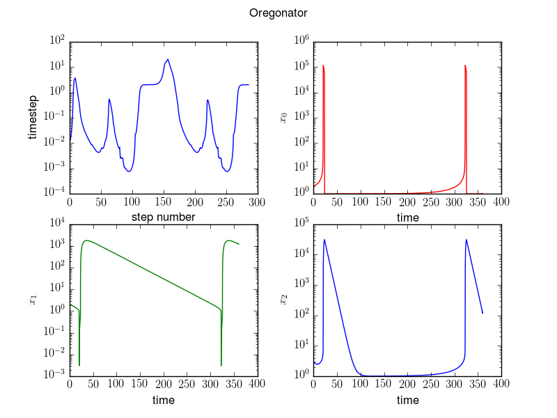
For these systems, it is best to use adaptive step size for the time integrators or time-stepping scheme.

• Using an adaptive stepsize is of particular importance when there is a large variation in the size of the derivative.

• Adaptive time step means that you decrease your time step when the physical system you are trying to simulate has rapid variation dynamics, and larger time steps when your solution changes more slowly and is more stable.