13) Newton methods

Last time¶

• Convergence classes

• Intro to Newton methods

Today¶

1. Newton-Raphson Method
   1.1 An implementation

2. Convergence of fixed-point (by mean value theorem)

3. Convergence of fixed-point (by Taylor series)

4. A fresh derivation of Newton’s method via convergence theory

Convergence classes¶

A convergent rootfinding algorithm produces a sequence of approximations $x_k$ such that

where $f(x_*) = 0$. For analysis, it is convenient to define the errors $e_k = x_k - x_*$. We say that an iterative algorithm is $q$-linearly convergent if

(The $q$ is for “quotient”.) A smaller convergence factor $\rho$ represents faster convergence. A slightly weaker condition ($r$-linear convergence or just linear convergence - the “r” here is for “root”) is that

for all sufficiently large $k$ when the sequence $\{\epsilon_k\}$ converges $q$-linearly to 0.

We saw that:

1. Newton-Raphson Method¶

Much of numerical analysis reduces to Taylor series, the approximation

centered on some reference point $x_0$.

In numerical computation, it is exceedingly rare to look beyond the first-order approximation

Since $\tilde f_{x_0}(x)$ is a linear function, we can explicitly compute the unique solution of $\tilde f_{x_0}(x) = 0$ as

This is Newton’s Method (aka Newton-Raphson or Newton-Raphson-Simpson) for finding the roots of differentiable functions.

1.1 An implementation¶

That’s really fast!¶

• 10 digits of accuracy in 4 iterations.

• How is this convergence test different from the one we used for bisection?

• How can this break down?

2. Convergence of fixed-point (by mean value theorem)¶

Consider the iteration

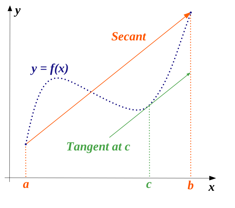
where $g$ is a continuously differentiable function. Suppose that there exists a fixed point $x_* = g(x_*)$. By the mean value theorem, we have that

for some $c_k$ between $x_k$ and $x_*$.

Taking absolute values,

which converges to zero if $|g'(c_k)| < 1$.

3. Convergence of fixed-point (by Taylor series)¶

Consider the iteration

where $g$ is a continuously differentiable function. Suppose that there exists a fixed point $x_* = g(x_*)$. There exists a Taylor series at $x_*$,

and thus

In terms of the error $e_k = x_k - x_*$,

Poll 13.1: Convergence class of the fixed-point method¶

Is this convergence:

• A=q-linear

• B=r-linear

• C=neither

Recall the definition of q-linear convergence

So, clearly, we need

to have convergence of the fixed-point iteration method. Otherwise, it diverges.

Aside:¶

• Big $O$ (“big oh”) notation

Limit $n\to\infty$:¶

We’d say an algorithm costs $O(n^2)$ if its running time on input of size $n$ is less than $c n^2$ for some constant $c$ and sufficiently large $n$.

Sometimes we write $\operatorname{cost}(\texttt{algorithm}, n) = O(n^2)$ or (preferably) $\operatorname{cost}(\texttt{algorithm}) \in O(n^2)$.

Note that $O(\log n) \subset O(n) \subset O(n\log n) \subset O(n^2) \subset \dotsb$.

We say the algorithm is in $\Theta(n^2)$ (“big theta”) if

for some positive constants $c_1,c_2$ and sufficiently large $n$.

Limit $h \to 0$:¶

In numerical analysis, we often have a small real number, and now the definitions take the limit as the small number goes to zero. So we say a term in an expression is in $O(h^2)$ if

Big $O$ terms can be manipulated as

Example of a fixed-point iteration¶

We wanted to solve $\cos x - x = 0$, which occurs when $g(x) = \cos x$ is a fixed point.

Verifying fixed-point method convergence theory¶

Reading: FNC Fixed-point iteration¶

Plotting Newton convergence¶

Poll 13.2: Convergence of Newton’s method¶

Is this convergence:

• A=q-linear

• B=r-linear

• C=neither?

Formulations are not unique (constants):¶

If $x = g(x)$ then

for any constant $c \ne 0$. Can we choose $c$ to make $\lvert g_2'(x_*) \rvert$ small?

Formulations are not unique (functions)¶

If $x = g(x)$ then

for any smooth $h(x) \ne 0$. Can we choose $h(x)$ to make $\lvert g_3'(x) \rvert$ small?

Exercise 13.1:¶

Compute $|g_3'(x_*)|$.

Note:

• We don’t know $g'(x_*)$ in advance because we don’t know $x_*$ yet.

• This method converges very fast

• We actually just derived Newton’s method.

4. A fresh derivation of Newton’s method via convergence theory¶

• A rootfinding problem $f(x) = 0$ can be converted to a fixed point problem

  $$x = x + f(x) =: g(x)$$

  (23)

  but there is no guarantee that $g'(x_*) = 1 + f'(x_*)$ will have magnitude less than 1.

• Problem-specific algebraic manipulation can be used to make $|g'(x_*)|$ small.

• $x = x + h(x) f(x)$ is also a valid formulation for any $h(x)$ bounded away from 0.

• Can we choose $h(x)$ such that

  $$g'(x) = 1 + h'(x) f(x) + h(x) f'(x) = 0$$

  (24)

  when $f(x) = 0$?

In other words,

Quadratic convergence!¶

• What does it mean that $g'(x_*) = 0$?

• It turns out that Newton’s method has locally quadratic convergence to simple roots,

  $$\lim_{k \to \infty} \frac{|e_{k+1}|}{|e_k|^2} < \infty.$$

  (27)

• “The number of correct digits doubles each iteration.”

• Now that we know how to make a good guess accurate, the effort lies in getting a good starting guess.

Rootfinding summary and outlook¶

• Newton methods are immensely successful

  • Convergence theory is local; we need good initial guesses

  • Computing the derivative $f'(x)$ is intrusive (and can be error-prone)

    • Avoided by secant methods (approximate the derivative)

    • Algorithmic or numerical differentiation can also be used instead of computing the derivative by hand

  • Bisection is robust when conditions are met

  • When does Newton diverge?

• More topics

  • Do we find all the roots?

  • Times when Newton converges slowly

Exercise 13.2:¶

1. Solve the fixed point iteration $g(x_n) = (2+{(x_n - 2)}^2)$, up to a tolerance 10^-6 or maximum number of iterations $N=50$, with (a) $x_0 = 2.8$, (b) $x_0 = 3.1$. Which execution is better? And why?

2. Solve the fixed point iteration $g(x_n) = (2+{(x_n - 2)}^3)$, up to a tolerance 10^-6 or maximum number of iterations $N=50$, with (a) $x_0 = 2.8$, (b) $x_0 = 3.1$. Which execution is better? And why?