34) Differentiation#
Last time#
Gradient descent
Nonlinear models
Today#
Computing derivatives
1.1 Numeric
1.2 Analytic by hand
1.3 Algorithmic (automatic) differentiationRecap on Finite Differences
Ill-conditioned optimization
1. Computing derivatives#
We know the definition of the difference quotient from Calculus:
How should we choose \(h\)?
Taylor series#
Classical accuracy analysis assumes that functions are sufficiently smooth, meaning that derivatives exist and Taylor expansions are valid within a neighborhood. In particular,
The big-\(O\) notation is meant in the limit \(h\to 0\). Specifically, a function \(g(h) \in O(h^p)\) (sometimes written \(g(h) = O(h^p)\)) when there exists a constant \(C\) such that
Rounding error#
We have an additional source of error, rounding error, which comes from not being able to compute \(f(x)\) or \(f(x+h)\) exactly, nor subtract them exactly. Suppose that we can, however, compute these functions with a relative error on the order of \(\epsilon_{\text{machine}}\). This leads to
Tedious error propagation#
where we have assumed that \(h \ge \epsilon_{\text{machine}}\). This error becomes large (relative to \(f'\) – we are concerned with relative error after all).
What can be problematic:
\(f\) is large compared to \(f'\)
\(x\) is large
\(h\) is too small
Automatic step size selection#
Reference: Numerical Optimization.
Walker and Pernice
Dennis and Schnabel
diff(f, x; h=1e-8) = (f(x+h) - f(x)) / h

function diff_wp(f, x; h=1e-8)
    """Diff using Walker and Pernice (1998) choice of step"""
    h *= (1 + abs(x))
    (f(x+h) - f(x)) / h
end

x = 1000
diff_wp(sin, x) - cos(x)
-4.139506408429305e-6
1.1 Symbolic differentiation#
using Pkg
Pkg.add("Symbolics")

using Symbolics

@variables x
Dx = Differential(x)

y = sin(x)
Dx(y)
Resolving package versions...
  No Changes to `~/.julia/environments/v1.10/Project.toml`
  No Changes to `~/.julia/environments/v1.10/Manifest.toml`
expand_derivatives(Dx(y))
Awesome, what about products?
y = x
for _ in 1:2
    y = cos(y^pi) * log(y)
end
expand_derivatives(Dx(y))
The size of these expressions can grow exponentially
1.2 Hand-coding (analytic) derivatives#
function f(x)
    y = x
    for _ in 1:2
        a = y^pi
        b = cos(a)
        c = log(y)
        y = b * c
    end
    y
end

f(1.9), diff_wp(f, 1.9)
(-1.5346823414986814, -34.032439961925064)
function df(x, dx)
    y = x
    dy = dx
    for _ in 1:2
        a = y ^ pi
        da = pi * y^(pi - 1) * dy
        b = cos(a)
        db = -sin(a) * da
        c = log(y)
        dc = dy / y
        y = b * c
        dy = db * c + b * dc
    end
    y, dy
end

df(1.9, 1)
(-1.5346823414986814, -34.032419599140475)
We can go the other way#
We can differentiate a composition \(h(g(f(x)))\) as
What we’ve done above is called “forward mode”, and amounts to placing the parentheses in the chain rule like
The expression means the same thing if we rearrange the parentheses,
which we can compute in reverse order via
A reverse mode example#
function g(x)
    a = x^pi
    b = cos(a)
    c = log(x)
    y = b * c
    y
end
(g(1.4), diff_wp(g, 1.4))
(-0.32484122107701546, -1.2559760384500684)
function gback(x, y_)
    a = x^pi
    b = cos(a)
    c = log(x)
    y = b * c
    # backward pass
    c_ = y_ * b
    b_ = c * y_
    a_ = -sin(a) * b_
    x_ = 1/x * c_ + pi * x^(pi-1) * a_
    x_
end
gback(1.4, 1)
-1.2559761698835525
1.3 Automatic differentiation: Zygote.jl#
using Pkg
Pkg.add("Zygote")

import Zygote
Resolving package versions...
  No Changes to `~/.julia/environments/v1.10/Project.toml`
  No Changes to `~/.julia/environments/v1.10/Manifest.toml`
Zygote.gradient(f, 1.9)
(-34.03241959914049,)
g(x) = exp(x) + x^2
@code_llvm Zygote.gradient(g, 1.9)
;  @ /home/vbarra/.julia/packages/Zygote/55SqB/src/compiler/interface.jl:152 within `gradient`
define [1 x double] @julia_gradient_4762(double %0) #0 {
top:
;  @ /home/vbarra/.julia/packages/Zygote/55SqB/src/compiler/interface.jl:153 within `gradient`
; ┌ @ /home/vbarra/.julia/packages/Zygote/55SqB/src/compiler/interface.jl:94 within `pullback` @ /home/vbarra/.julia/packages/Zygote/55SqB/src/compiler/interface.jl:96
; │┌ @ In[11]:1 within `g`
; ││┌ @ /home/vbarra/.julia/packages/Zygote/55SqB/src/compiler/interface2.jl:81 within `_pullback`
; │││┌ @ /home/vbarra/.julia/packages/Zygote/55SqB/src/compiler/interface2.jl within `macro expansion`
; ││││┌ @ /home/vbarra/.julia/packages/Zygote/55SqB/src/compiler/chainrules.jl:234 within `chain_rrule`
; │││││┌ @ /home/vbarra/.julia/packages/ChainRulesCore/U6wNx/src/rules.jl:138 within `rrule` @ /home/vbarra/.julia/packages/ChainRules/166sf/src/rulesets/Base/fastmath_able.jl:56
        %1 = call double @j_exp_4764(double %0)
; └└└└└└
;  @ /home/vbarra/.julia/packages/Zygote/55SqB/src/compiler/interface.jl:154 within `gradient`
; ┌ @ /home/vbarra/.julia/packages/Zygote/55SqB/src/compiler/interface.jl:97 within `#88`
; │┌ @ In[11]:1 within `g`
; ││┌ @ /home/vbarra/.julia/packages/Zygote/55SqB/src/compiler/chainrules.jl:222 within `ZBack`
; │││┌ @ /home/vbarra/.julia/packages/Zygote/55SqB/src/lib/number.jl:12 within `literal_pow_pullback`
; ││││┌ @ promotion.jl:423 within `*` @ float.jl:411
       %2 = fmul double %0, 2.000000e+00
; │└└└└
; │┌ @ /home/vbarra/.julia/packages/Zygote/55SqB/src/lib/lib.jl:9 within `accum`
; ││┌ @ float.jl:409 within `+`
     %3 = fadd double %2, %1
; └└└
;  @ /home/vbarra/.julia/packages/Zygote/55SqB/src/compiler/interface.jl:155 within `gradient`
  %unbox3.fca.0.insert = insertvalue [1 x double] zeroinitializer, double %3, 0
  ret [1 x double] %unbox3.fca.0.insert
}
How does Zygote work?#
square(x) = x^2
@code_llvm square(1.5)
;  @ In[12]:1 within `square`
define double @julia_square_4786(double %0) #0 {
top:
; ┌ @ intfuncs.jl:332 within `literal_pow`
; │┌ @ float.jl:411 within `*`
    %1 = fmul double %0, %0
    ret double %1
; └└
}
@code_llvm Zygote.gradient(square, 1.5)
;  @ /home/vbarra/.julia/packages/Zygote/55SqB/src/compiler/interface.jl:152 within `gradient`
define [1 x double] @julia_gradient_4790(double %0) #0 {
top:
;  @ /home/vbarra/.julia/packages/Zygote/55SqB/src/compiler/interface.jl:154 within `gradient`
; ┌ @ /home/vbarra/.julia/packages/Zygote/55SqB/src/compiler/interface.jl:97 within `#88`
; │┌ @ In[12]:1 within `square`
; ││┌ @ /home/vbarra/.julia/packages/Zygote/55SqB/src/compiler/chainrules.jl:222 within `ZBack`
; │││┌ @ /home/vbarra/.julia/packages/Zygote/55SqB/src/lib/number.jl:12 within `literal_pow_pullback`
; ││││┌ @ promotion.jl:423 within `*` @ float.jl:411
       %1 = fmul double %0, 2.000000e+00
; └└└└└
;  @ /home/vbarra/.julia/packages/Zygote/55SqB/src/compiler/interface.jl:155 within `gradient`
  %unbox2.fca.0.insert = insertvalue [1 x double] zeroinitializer, double %1, 0
  ret [1 x double] %unbox2.fca.0.insert
}
Kinds of algorithmic differentation#
Source transformation: Fortran code in, Fortran code out
Duplicates compiler features, usually incomplete language coverage
Produces efficient code
Operator overloading: C++ types
Hard to vectorize
Loops are effectively unrolled/inefficient
Just-in-time compilation: tightly coupled with compiler
JIT lag
Needs dynamic language features (JAX) or tight integration with compiler (Zygote, Enzyme)
Some sharp bits in Python’s JAX
Forward or reverse?#
It all depends on the shape.
If you have one input, many outputs: use forward mode
“One input” can be looking in one direction
If you have many inputs, one output: use reverse mode
Will need to traverse execution backwards (“tape”)
Hierarchical checkpointing
What about square cases (same number of input/output)? Forward is usually a bit more efficient.
Can you differentiate an algorithm?#
Examples:
Optimization: Input \(c\), output \(x\) such that \(f(x,c)=0\)
Finding eigenvalues/eigenvectors: Input \(A\), output \(\lambda\) such that \(Ax = \lambda x\) for some nonzero vector
2. Recap on Finite Differences#
Finite Differences#
To define derivatives, we use Taylor’s expansion:
Similarly,
Consider a uniformly discretized domain (with uniform \(h \equiv \Delta x\) subintervals)
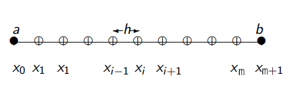
We can define the first-order derivative at the point \(x_i\) using the forward difference:
this is a first-order approximation.
Similarly, we can define the first-order derivative at the point \(x_i\) using the backward difference:
this is a first-order approximation.
If we use one point to the right of \(x_i\) and one point to the left of \(x_i\) we have a centered difference approximation for the first-order derivative at the point \(x_i\) using the centered difference:
this is a second-order approximation.
Thus we note that the centered difference approximates the first derivative with respect to \(x\) more accurately than either of the one-sided differences, \(O( \Delta x^2 )\) versus \(\Delta x\).
We can now define a second-order derivative, at the point \(x_i\) using a centered difference formula:
3. Ill-conditioned optimization#
Recall that the computation of the gradient of the loss function \(L\) requires the Jacobian, denoted by \(J\), of the model \(f\) differentiated w. r. t. the constants \(c\).
We can find the constants \(c\) for which \(g(c) = 0\) using a Newton method
The Hessian requires the second derivative of \(f\), which can cause problems.
Newton-like methods for optimization#
We want to solve
Update
Gauss-Newton: \(H = J^T J\)
Levenberg-Marquardt: \(H = J^T J + \alpha J\)
Outlook on optimization#
The optimization problem can be solved using a Newton method. It can be onerous to implement the needed derivatives.
The Gauss-Newton method is often more practical than Newton while being faster than gradient descent, though it lacks robustness.
The Levenberg-Marquardt method provides a sort of middle-ground between Gauss-Newton and gradient descent.
Many globalization techniques are used for models that possess many local minima.
One pervasive approach is stochastic gradient descent, where small batches (e.g., 1, 10 or 20) are selected randomly from the corpus of observations (500 in the example we’ve seen with many realizations), and a step of gradient descent is applied to that reduced set of observations. This helps to escape saddle points and weak local minima.
Among expressive models \(f(x,c)\), some may converge much more easily than others. Having a good optimization algorithm is essential for nonlinear regression with complicated models, especially those with many parameters \(c\).
Classification is a very similar problem to regression, but the observations \(y\) are discrete, thus, in this case
models \(f(x,c)\) must have discrete output
the least squares loss function is not appropriate.
Reading: Why momentum really works